Chapter 4 SQL
The questing beast.
Sir Thomas Malory, Le Morte D’Arthur, 1470
Structured query language
Structured query language (SQL) is widely used as a relational database language, and SQL skills are essential for data management in a world that is increasingly reliant on database technology. SQL originated in the IBM Research Laboratory in San Jose, California. Versions have since been implemented by commercial database vendors and open source teams for a wide range of operating systems. Both the American National Standards Institute (ANSI) and the International Organization for Standardization (ISO) have designated SQL as a standard language for relational database systems.
SQL is a complete database language. It is used for defining a relational database, creating views, and specifying queries. In addition, it allows for rows to be inserted, updated, and deleted. In database terminology, it is both a data definition language (DDL), a data manipulation language (DML), and a data control language (DCL). SQL, however, is not a complete programming language like Python, R, and Java. Because SQL statements can be embedded into general-purpose programming languages, SQL is often used in conjunction with such languages to create application programs. The embedded SQL statements handle the database processing, and the statements in the general-purpose language perform the necessary tasks to complete the application.
Data types
Some of the variety of data types that can be used are depicted in the following figure and described in more detail in the following pages.
Data types
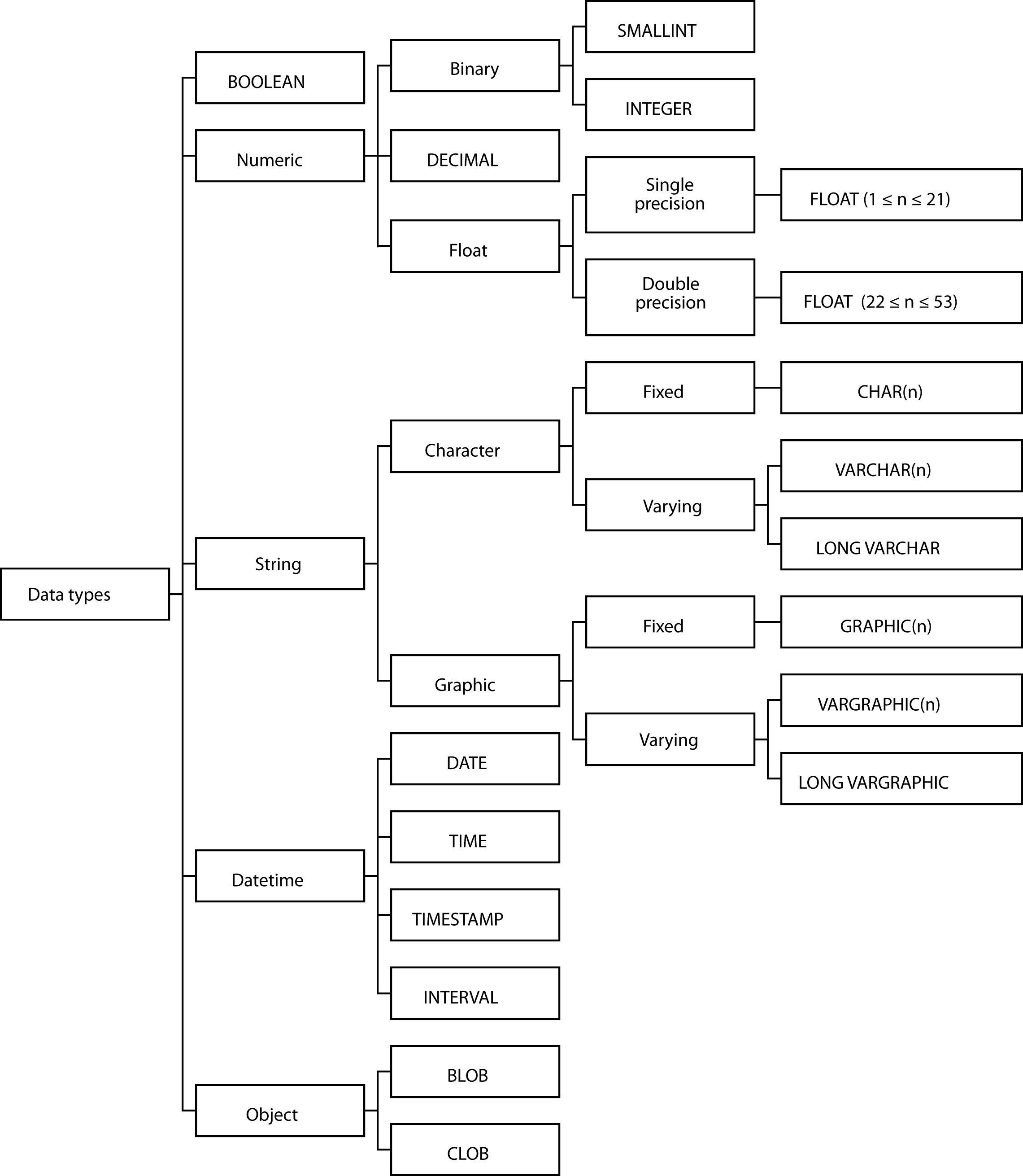
SMALLINT and INTEGER
Most commercial computers have a 32-bit word, where a word is a unit of storage. An integer can be stored in a full word or half a word. If it is stored in a full word (INTEGER), then it can be 31 binary digits in length. If half-word storage is used (SMALLINT), then it can be 15 binary digits long. In each case, one bit is used for the sign of the number. A column defined as INTEGER can store a number in the range -231 to 231-1 or -2,147,483,648 to 2,147,483,647. A column defined as SMALLINT can store a number in the range -215 to 215-1 or -32,768 to 32,767. Just remember that INTEGER is good for ±2 billion and SMALLINT for ±32,000.
FLOAT
Scientists often deal with numbers that are very large (e.g., Avogadro’s number is 6.02252×10²³) or very small (e.g., Planck’s constant is 6.6262×10⁻³⁴ joule sec). The FLOAT data type is used for storing such numbers, often referred to as floating-point numbers. A single-precision floating-point number requires 32 bits and can represent numbers in the range -7.2×1075 to -5.4×10-79, 0, 5.4×10-79 to 7.2×1075 with a precision of about 7 decimal digits. A double-precision floating-point number requires 64 bits. The range is the same as for a single-precision floating-point number. The extra 32 bits are used to increase precision to about 15 decimal digits.
In the specification FLOAT(n), if n is between 1 and 21 inclusive, single-precision floating-point is selected. If n is between 22 and 53 inclusive, the storage format is double-precision floating-point. If n is not specified, double-precision floating-point is assumed.
DECIMAL
Binary is the most convenient form of storing data from a computer’s perspective. People, however, work with a decimal number system. The DECIMAL data type is convenient for business applications because data storage requirements are defined in terms of the maximum number of places to the left and right of the decimal point. To store the current value of an ounce of gold, you would possibly use DECIMAL(6,2) because this would permit a maximum value of $9,999.99. Notice that the general form is DECIMAL(p,q), where p is the total number of digits in the column, and q is the number of digits to the right of the decimal point.
CHAR and VARCHAR
Nonnumeric columns are stored as character strings. A person’s family name is an example of a column that is stored as a character string. CHAR(n) defines a column that has a fixed length of n characters, where n can be a maximum of 255.
When a column’s length can vary greatly, it makes sense to define the field as VARCHAR. A column defined as VARCHAR consists of two parts: a header indicating the length of the character string and the string. If a table contains a column that occasionally stores a long string of text (e.g., a message field), then defining it as VARCHAR makes sense. VARCHAR can store strings up to 65,535 characters long.
Why not store all character columns as VARCHAR and save space? There is a price for using VARCHAR with some relational systems. First, additional space is required for the header to indicate the length of the string. Second, additional processing time is required to handle a variable-length string compared to a fixed-length string. Depending on the RDBMS and processor speed, these might be important considerations, and some systems will automatically make an appropriate choice. For example, if you use both data types in the same table, MySQL will automatically change CHAR into VARCHAR for compatibility reasons.
There are some columns where there is no trade-off because all possible entries are always the same length. Canadian postal codes, for instance, are always six characters (e.g., the postal code for Ottawa is K1A0A1).
Data compression is another approach to the space wars problem. A database can be defined with generous allowances for fixed-length character columns so that few values are truncated. Data compression can be used to compress the file to remove wasted space. Data compression, however, is slow and will increase the time to process queries. You save space at the cost of time, and save time at the cost of space. When dealing with character fields, the database designer has to decide whether time or space is more important.
Times and dates
Columns that have a data type of DATE are stored as yyyymmdd (e.g., 2022-11-04 for November 4, 2022). There are two reasons for this format. First, it is convenient for sorting in chronological order. The common American way of writing dates (mmddyy) requires processing before chronological sorting. Second, the full form of the year should be recorded for exactness.
For similar reasons, it makes sense to store times in the form hhmmss with the understanding that this is 24-hour time (also known as European time and military time). This is the format used for data type TIME.
Some applications require precise recording of events. For example, transaction processing systems typically record the time a transaction was processed by the system. Because computers operate at high speed, the TIMESTAMP data type records date and time with microsecond accuracy. A timestamp has seven parts: year, month, day, hour, minute, second, and microsecond. Date and time are defined as previously described (i.e., yyyymmdd and hhmmss, respectively). The range of the microsecond part is 000000 to 999999.
Although times and dates are stored in a particular format, the formatting facilities that generally come with a RDBMS usually allow tailoring of time and date output to suit local standards. Thus for a U.S. firm, date might appear on a report in the form mm/dd/yy; for a European firm following the ISO standard, date would appear as yyyy-mm-dd.
SQL-99 introduced the INTERVAL data type, which is a single value expressed in some unit or units of time (e.g., 6 years, 5 days, 7 hours).
BLOB (binary large object)
BLOB is a large-object data type that stores any kind of binary data. Binary data typically consists of a saved spreadsheet, graph, audio file, satellite image, voice pattern, or any digitized data. The BLOB data type has no maximum size.
CLOB (character large object)
CLOB is a large-object data type that stores any kind of character data. Text data typically consists of reports, correspondence, chapters of a manual, or contracts. The CLOB data type has no maximum size.
❓ Skill builder
What data types would you recommend for the following?
A book’s ISBN
A photo of a product
The speed of light (2.9979 × 10⁸ meters per second)
A short description of an animal’s habitat
The title of a Japanese book
A legal contract
The status of an electrical switch
The date and time a reservation was made
An item’s value in euros
The number of children in a family
Scalar functions
Most implementations of SQL include functions that can be used in arithmetic expressions, and for data conversion or data extraction. The following sampling of these functions will give you an idea of what is available. You will need to consult the documentation for your version of SQL to determine the functions it supports. For example, Microsoft SQL Server has more than 100 additional functions.
Some examples of SQL’s built-in scalar functions
| Function | Description |
|---|---|
| CURRENT_DATE() | Retrieves the current date |
| EXTRACT(date_time_part FROM expression) | Retrieves part of a time or date (e.g., YEAR, MONTH, DAY, HOUR, MINUTE, or SECOND) |
| SUBSTRING(str, pos, len) | Retrieves a string of length len starting at position pos from string str |
Some examples for you to run
SELECT extract(day) FROM CURRENT_DATE());SELECT SUBSTRING(`person first`, 1,1), `person last` FROM person;A vendor’s additional functions can be very useful. Remember, though, that use of a vendor’s extensions might limit portability.
Formatting
You will likely have noticed that some queries report numeric values with a varying number of decimal places. The FORMAT function gives you control over the number of decimal places reported, as illustrated in the following example where yield is reported with two decimal places.
SELECT shrfirm, shrprice, shrqty, FORMAT(shrdiv/shrprice*100,2)
  AS yield
    FROM share;
When you use format you create a string, but you often want to sort on the numeric value of the formatted field. The following example illustrates how to do this.
SELECT shrfirm, shrprice, shrqty, FORMAT(shrdiv/shrprice*100,2)
  AS yield FROM share
      ORDER BY shrdiv/shrprice*100 DESC;
Run the following code to see the difference.
SELECT shrfirm, shrprice, shrqty, FORMAT(shrdiv/shrprice*100,2)
  AS yield FROM share
      ORDER BY yield DESC;
Data manipulation
SQL supports four DML statements—SELECT, INSERT, UPDATE, and DELETE. Most attention is focussed on SELECT because of the variety of ways in which it can be used. First, we need to understand why we must qualify column names and temporary names.
Qualifying column names
Ambiguous references to column names are avoided by qualifying a column
name with its table name, especially when the same column name is used
in several tables. Clarity is maintained by prefixing the column name
with the table name. The following example demonstrates qualification of
the natcode, which appears in both stock and nation.
SELECT stkfirm, stkprice FROM stock JOIN nation
    ON stock.natcode = nation.natcode;
SELECT
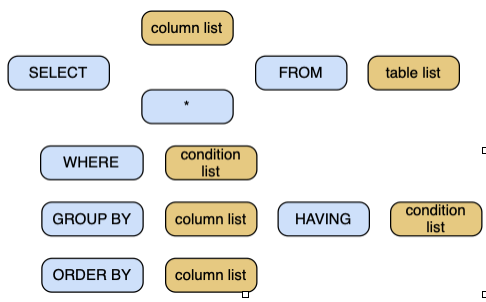
The SELECT statement is by far the most interesting and challenging of the four DML statements. It reveals a major benefit of the relational model: powerful interrogation capabilities. It is challenging because mastering the power of SELECT requires considerable practice with a wide range of queries. The major varieties of SELECT are presented in this section.
The general format of SELECT is
SELECT [DISTINCT] item(s) FROM table(s)
    [WHERE condition]
    [GROUP BY column(s)] [HAVING condition]
    [ORDER BY column(s)];
Alternatively, we can diagram the structure of SELECT.
Structure of SELECT
Simple subquery
A subquery is a query within a query. There is a SELECT statement nested inside another SELECT statement. Simple subqueries were used extensively in earlier chapters. For reference, here is a simple subquery used earlier:
SELECT stkfirm FROM stock
    WHERE natcode IN
        (SELECT natcode FROM nation
            WHERE natname = 'Australia');
Aggregate functions
SQL’s aggregate functions increase its retrieval power. These functions were covered earlier and are only mentioned briefly here for completeness. The five aggregate functions are shown in the following table. Nulls in the column are ignored in the case of SUM, AVG, MAX, and MIN. COUNT(*) does not distinguish between null and non-null values in a column. Use COUNT(columnname) to exclude a null value in columnname.
Aggregate functions
| Function | Description |
|---|---|
| COUNT | Counts the number of values in a column |
| SUM | Sums the values in a column |
| AVG | Determines the average of the values in a column |
| MAX | Determines the largest value in a column |
| MIN | Determines the smallest value in a column |
GROUP BY and HAVING
The GROUP BY clause is an elementary form of control break reporting and supports grouping of rows that have the same value for a specified column and produces one row for each different value of the grouping column. For example,
Report by nation the total value of stockholdings.
SELECT natname, SUM(stkprice*stkqty*exchrate) AS total
    FROM stock JOIN nation ON stock.natcode = nation.natcode
        GROUP BY natname;
The HAVING clause is often associated with GROUP BY. It can be thought of as the WHERE clause of GROUP BY because it is used to eliminate rows for a GROUP BY condition. Both GROUP BY and HAVING are dealt with in-depth in Chapter 4.
Nulls—much ado about missing information
Nulls are overworked in SQL because they can represent several situations. Null can represent unknown information. For example, you might add a new stock to the database, but lacking details of its latest dividend, you leave the field null. Null can be used to represent a value that is inapplicable. For instance, the employee table contains a null value in bossno for Alice because she has no boss. The value is not unknown; it is not applicable for that field. In other cases, null might mean “no value supplied” or “value undefined.” Because null can have multiple meanings, the client must infer which meaning is appropriate to the circumstances.
Do not confuse null with blank or zero, which are values. In fact, null is a marker that specifies that the value for the particular column is null. Thus, null represents no value.
The well-known database expert Chris Date has been outspoken in his concern about the confusion caused by nulls. His advice is that nulls should be explicitly avoided by specifying NOT NULL for all columns and by using codes to make the meaning of a value clear (e.g., “U” means “unknown,” “I” means “inapplicable,” and “N” means “not supplied”).
The future of SQL
Since 1986, developers of database applications have benefited from an SQL standard, one of the more successful standardization stories in the software industry. Although most database vendors have implemented proprietary extensions of SQL, standardization has kept the language consistent, and SQL code is highly portable. Standardization was relatively easy when focused on the storage and retrieval of numbers and characters. Objects have made standardization more difficult.
Summary
Structured Query Language (SQL), a widely used relational database language, has been adopted as a standard by ANSI and ISO. It is a data definition language (DDL), data manipulation language (DML), and data control language (DCL).
A base table is an autonomous, named table. A key is one or more columns identified as such in the description of a table or a referential constraint. SQL supports primary, foreign, and unique keys.
Numeric, string, date, or graphic data can be stored in a column. BLOB and CLOB are data types for large fields.
Ambiguous references to column names are avoided by qualifying a column name with its table name. A table or view can be given a temporary name that remains current for a query.
SELECT provides powerful interrogation facilities. The product of two tables is a new table consisting of all rows of the first table concatenated with all possible rows of the second table. Join creates a new table from two existing tables by matching on a column common to both tables. A subquery is a query within a query.
SQL’s aggregate functions increase its retrieval power. GROUP BY supports grouping of rows that have the same value for a specified column. The REXEXP clause supports pattern matching. SQL includes scalar functions that can be used in arithmetic expressions, data conversion, or data extraction. Nulls cause problems because they can represent several situations—unknown information, inapplicable information, no value supplied, or value undefined. Remember, a null is not a blank or zero.